Acceptance-rejection algorithm
This is one of my favourite introductory algorithm for sampling data from a distribution. A pre requisite basic knowledge about probability distribution, CDF and inverse CDF is necessary to follow the article.
A probability distribution gives the probability of having a random variable Y. To get Y from probability, a usual method is to find inverse CDF. There are several pdf whose inverse are difficult to obtain, does not exist or have no closed solution. Acceptance-Rejection method is used when it is not possible to find inverse CDF of a distribution, but we can get random variable (rv) using inverse of another similar distribution and say whether this particular rv can be used as if it was generated from our original distribution.
In acceptance rejection method, the idea is to find a probability distribution, \(g_y\), from which we can generate a random variable (rv) Y and able to tell whether this rv can be accepted for our target distribution, \(f_y\). The random variable Y is chosen in such a way that the \(g_y\) can be scaled to majorize \(f_y\) using some constant c; that is \(c.g_y(x)\geq f_y(x)\). The density \(g_y\) is known as majorizing density or proposal density and \(f_y\) is known as target density. The support of the target density must be contained in the support of proposal density. For density having infinite support, the majorizing density should also have infinite support. In the case of infinite support, it is critical that the majorizing density should not approach zero faster than the target density. It makes sense now as if there’s a region of the support of f that g can never touch, then that area will never get sampled.
Following is the Acceptance Rejection algorithm :
- Sample a rv Y \(\sim g_y(x)\) ( by taking inverse CDF. Remember, taking inverse of majorizing function should be easy)
- Sample from uniform distribution U \(\sim\) Unif(0,1).
- Reject Y if U > \(\frac{f_y(x)}{C.g_y(x)}\). Go to step 1.
- Else accept Y for \(f_y(x)\).
- Keep repeating the above step for desired number of samples.
Step 2 generates uniform probability between 0 and 1. In Step 3 but the ratio \(f_y(x)/g_y(x)\) is bounded by a constant c>0. c.g(x) acts as a envelope for the target function \(f_y\). I did not find much meaning of the ratio but one way to think about this fraction is that, it inherently implies that how many fraction of rv for \(f_y\) is included in c*\(g_y\). Step 3 implies that if the probability of generated point is lesser than probability generated by uniform distribution then accept that sample, which I find is a nice way to think about it. We need to maximize this fraction so that we can cover most of the points in \(g_y\) for \(f_y\). Moreover, larger C value will result into rejection of more samples so we need to find c as small as possible.
Example-1: Generating beta(2,7) distribution
#code by : Krzysztof Bartoszek
fgenbeta<-function(c){
    x<-NA
    num.reject<-0
    while (is.na(x)){
    y<-runif(1)
    u<-runif(1)
    if (u<=dbeta(y,2,7)/c){x<-y}
    else{num.reject<-num.reject+1}
    }
    c(x,num.reject)
}

y<-dbeta(seq(0,2,0.001),2,7)
c<-max(y)

mbetas1<-sapply(rep(c,10000),fgenbeta)
mbetas2<-sapply(rep(4,10000),fgenbeta)

par(mfrow=c(1,2))

hist(mbetas1[2,],col="black",breaks=100,xlab="",ylab="",freq=FALSE,main="");hist(mbetas2[2,],col=gray(0.8),breaks=100,xlab="",ylab="",freq=FALSE,main="",add=TRUE);legend("topright",pch=19,cex=1.2,legend=c("c=3.172","c=4"),col=c("black",gray(0.8)),bty="n")
hist(mbetas1[1,],col="black",breaks=100,xlab="",ylab="",freq=FALSE,main="",ylim=c(0,3.5));hist(mbetas2[1,],col=gray(0.8),breaks=100,xlab="",ylab="",freq=FALSE,main="",add=TRUE);points(seq(0,2,0.001),y,pch=19,cex=0.3,col=gray(0.4));abline(h=3.172554,lwd=3);legend("right",pch=19,cex=1.2,legend=c("c=3.172","c=4"),col=c("black",gray(0.8)),bty="n")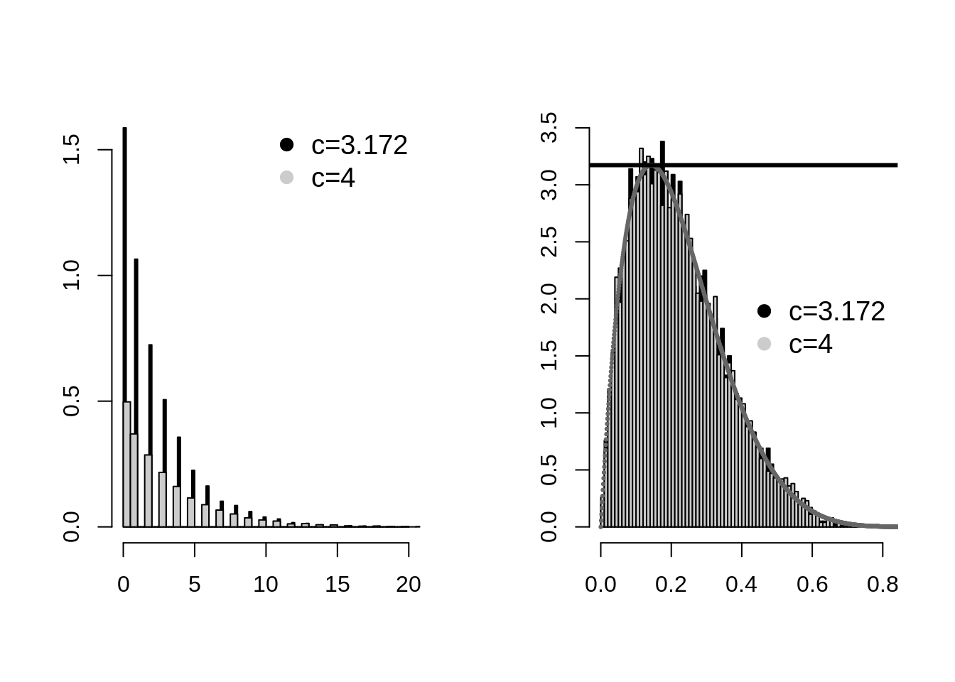
We can see from the above example that the larger value of c tends to reject more sample than low value of c. The black color shows that the samples of beta distribution was accepted more than that of gray color. In second picture one can see black lines even though it is in background which shows that lesser c values has lower rejection rate.
As an another example, let’s generate samples for normal distribution \(\mathcal{N(0,1)}\) using Laplace or double exponential distribution as proposal density DE(0, 1). Below are the given two distribution :
\[ \begin{aligned} g(x|\mu=0,\alpha=1) &= \frac{1}{2}* e^{-|x|} \hspace{40pt} :Laplace Distribution \\ f(x |\mu=0,\alpha=1) &= \frac{1}{\sqrt{2\pi}}* e^{\frac{-x^{2}}{2}} \hspace{24pt} :Normal Distribution \\ \end{aligned} \]
As I mentioned before that the ratio \(f_y(x)/g_y(x)\) is bounded by a constant c>0 and \(sup_x{f(x)/g(x))}\) \(\le\) c. Another way to imagine the above equation is that, this equation gives the probability of accepting the sample and we need to maximize the acceptance sample. So,
\[\begin{aligned} C&\geq \frac{f(x)}{g(x)} \\ C&\geq \frac{\sqrt{2}* e^{-\frac{x^2}{2}+|x|}}{\sqrt{\pi}} \end{aligned} \]
Then we differentiate the above ratio and equate to 0 to get the value of x which will give the value of C. On doing it, we get it as:
\[\frac{\sqrt{2}* e^{-\frac{x^2}{2}+|x|}}{\sqrt{\pi}} *(\frac{|x|}{x}-x) \]
Setting the above differential to zero we get the maximum value of above equation at x=1, value of C is obtained.
\[ C = \sqrt{\frac{2e}{\pi}} \]
The condition to accept RV generated from g(x) as RV for f(x) is : \[ \begin{aligned} U & \leq \frac{f(x)}{C*g(x)} \\ U &\leq 0.5*e^{\frac{x^2}{2} + |x|} \end{aligned} \]
Step 1 of equation is generating samples from Laplace distribution whose inverse can be found. This link gives how to find the inverse.
Below is the complete code for acceptance-rejection:
#author: Naveen gabriel
accept_reject <- function(sam) {
    f_x <- c()
    cnt <- 1
    while(cnt<=sam){
        U <- runif(1,0,1)
        r_x <- ifelse(U<0.5, log(2*U), -log(2-(2*U)))  #generate a random variable from laplace distribution

        uni <- runif(1)
        frac <- exp(-(r_x^2)/2 + abs(r_x) - 0.5)  #value of f(X)/c(g(X))

        if(uni<=frac){
            f_x[cnt]<- r_x
            cnt <- cnt+1
        }
        total <<- total + 1
    }

return(f_x)
}

n = 2000
total <-0
values <- accept_reject(n)
normal_dist <- rnorm(2000,0,1)

compare_data <- cbind(values,normal_dist)
compare_data <- as.data.frame(compare_data)

colnames(compare_data) <- c("Accept_Rejection","normal_dist")
We can see that the normal distribution generated by acceptance rejection method is nearly same as distribution generated by rnorm.
ggplot(compare_data) + geom_histogram(aes(Accept_Rejection,fill="Accept_Rejection"),alpha=0.4) + geom_histogram(aes(normal_dist,fill ="normal_dist"), alpha =0.5) + labs(title="Histograms of two distribution", x = "Histograms")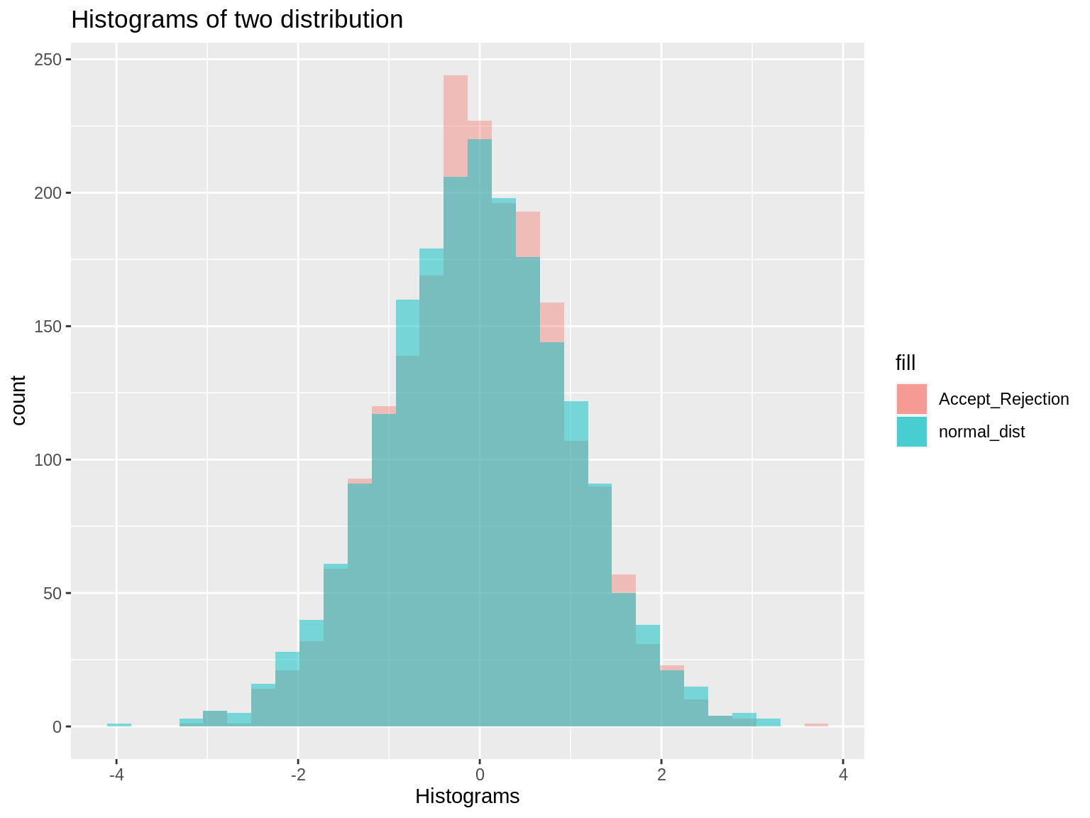
One property of the rejection sampling algorithm is that the number of draws we need to take from the candidate density g before we accept a candidate is a geometric random variable with success probability 1/c. Hence, the expected rejection rate is equal to: \[1 - \frac{1}{c} = 0.2398264\]
The average rejection rate is :
\[1 - \frac{2000}{total}\]
Where total is the total number of iterations required to generate 2000 samples. Our average rejection rate is nearly equal to expected rejection rate.
## The average rejection rate is : 0.2421372You might be thinking why we need sampling method, that too generating random samples from probability. Imagine you have dataset where there are missing values and you might know a distribution from which the samples can be generated. But taking the inverse of that distribution might be too difficult. In that case we can use this method. It might feel weird to do this process because we don’t encounter it while doing sampling. Many known densities (exponential, normal, beta etc) have library methods that generate samples using one of different sampling method. Unlike inverse CDF, this method can be extend to multivariate random variables. If the random variable is of a reasonably low dimension (less than 10?), then rejection sampling is a plausible general approach. But keep in mind that as the number of dimension increase the rate of rejection increases.
There are different flavors of rejection sampling like Squeezed rejection sampling, adaptive rejection sampling etc. The acceptance-rejection method can be generalized to the Metropolis–Hastings algorithm which is a type of Markov chain Monte Carlo simulation. Below are some of the awesome link to understand more of this method:
- Columbia university notes
- Stack overflow
- Rejection sampling (RS) technique, suggested first by John von Neumann in 1951.